
Darkmux Genesis II: Charting the Wake
Faster local AI on Apple Silicon — and the receipts. One setting that halved my elapsed time, the agent behavior single-number benchmarks can't capture, and three runtime bugs I filed along the way.

Where this picks up
Part 1 was the casual comparison: which local-AI model felt right for agentic work on Apple Silicon? Same task, same machine, see what each one did. The data was real and the conclusions held under what I tested.
But casual comparison raises more questions than it settles. Why did performance vary so much between identical runs? Was the configuration I’d settled on actually optimal, or just locally good? Was the summarization layer pulling its weight, or just adding overhead? The work needed to go deeper and more scientific. Otherwise I’d never get the speed and quality I wanted out of this machine.
Part 2 is what those questions grew into. Single-variable isolation, multi-run distributions, a planted-information probe, three runtime bugs that only methodical work surfaces. Same hardware, same models — different rigor. The kind that earns conclusions by holding every variable still while one thing changes.
This article runs longer than Part 1. The reason is that the methodical version of the work has its own arc — each finding is the answer to a question Part 1’s casual comparison couldn’t have asked yet. I’m publishing the arc, not just the endpoints.
Some of what follows is technical. I’ll keep the body human-readable and put the deep specifics in three short appendices for operators who want the receipts.
The notebook, and where it came from
Junior year of Electrical Engineering. Each EE lab was a week of prep and one full day of execution, graded on theory, hypothesis, design, and simulator runs during prep. On lab day, that preparation was tested under time pressure. The notes were the difference between an A and “works on paper.” All of it went into a hardcover lab notebook — on a once-a-week cadence — and the notebook was a large portion of the grade. Steps, formulas, results, every change. MATLAB diagrams printed, cut with scissors, taped in. Clear masking tape, edges fully sealed so the paper wouldn’t fray. Captions on every figure. Missing a required element cost points. Past entries kept becoming load-bearing. A circuit you’d designed, prototyped, and tested three weeks earlier was suddenly the reference for what you were trying to design today. Technology builds on documented foundations; new work can only stand on what came before if the past is accessible.
I used the same discipline for agentic AI on Apple Silicon. I kept a markdown lab notebook at the top of my project directory and made two rules:
Date-stamp every entry, even the trivial ones. Time gets compressed in memory; the notebook is the only honest record of what happened when.
Numbered “Eureka” index at the top. When a later session invalidated an earlier conclusion, the original entry got pruned to a one-line pointer and the corrected truth went into the index with a number.
By the end of the work covered in this article, that index had seven home-run entries.
A week chasing the wrong ghost
The first big lesson was a debugging story. It cost me a week.
The symptom was specific: long sessions — the kind where the AI assistant works through thirty or more steps, reading files, editing code, running tests — would chug along fine for a while and then suddenly fail. The OpenClaw + LMStudio harness would technically end without error, but the assistant’s last response was cut off mid-thought, and the closing report I’d asked for — confirming the work was done and the run exited cleanly — never appeared.
I spent four sessions hunting the prompt. Maybe my custom instructions contradicted my project notes. Maybe my safety reminders were fighting my work-style preferences. Maybe a tool’s output was malformed. Each theory produced a “fix” that worked on the next short test and failed on the next long one.
The actual cause wasn’t where I was looking. It was much earlier in the chain — in how the runtime had been told to talk to the model.
Earlier in the project, I’d configured the runtime with a context window size. LMStudio had loaded the model with a different size. Neither system warned me that the numbers disagreed. Conversations would grow, the runtime stayed calm, and then the model would suddenly hit its real limit and refuse the next request. But only when the conversation crossed that real limit — which is exactly when the symptom showed up.
This is the kind of misconfiguration most operators never find. The error doesn’t blame the right thing — the failing dispatch looks like the model itself is broken or the laptop is out of RAM. Most users walk away from local AI at this point. This article gives you somewhere else to look first.
The fix was one number. Tell the runtime the truth about how much room the model actually has. Six characters changed in a config file, and a week of failing dispatches resolved.
Lesson, written in my notebook the same night:
When a bug is conditional on workload size, the cause is almost certainly in the runtime’s belief about its resource limits, not the prompt content. Resource-debug, don’t content-debug.
The notebook made the pattern visible by accumulating 63 dated entries of deliberate experimentation. Cross-checking across them surfaced four with the same shape: short tests fine, long tests broken. I’d been treating each as a unique mystery.
If you want to check whether your own setup has the same calibration drift, ask your AI assistant:
Hey Claude: run
lms ps --jsonto see what’s loaded, then read my~/.openclaw/openclaw.jsonproviders list. Tell me whether thecontextWindowregistered for the loaded model matches the actually-loaded context length. If they’re out of sync, give me the one-line fix.
What the runtime won’t tell you about compaction
I’d run OpenClaw (v2026.5.4, an open-source agent runtime for local-LLM dispatch) on a frontier setup earlier in the project. The default config worked. I never touched compaction settings; didn’t know they existed. Switching to gpt-oss felt like it should be a no-op — same OpenClaw, same agent loop, just a local OpenAI variant. The first heavy dispatch failed.
The easy conclusions were wrong but rational: the model is garbage, local AI isn’t ready, OpenClaw doesn’t support OSS models. None of those were true. The local stack exposes a layer of tuning that frontier providers handle for you — and OpenClaw deliberately leaves the depth in source rather than wrapping it in settings most users would never need to touch. That’s the OSS contract working as designed: lean default surface, full tuning depth available to whoever digs. Compaction is one of those knobs.
Compaction — the system summarizing older conversation turns to free room when context fills — is a critical performance factor in the runtime, and most likely in any agent system with a similar summarization step. Each compaction is a discrete event: the runtime pauses the conversation, summarizes, and resumes.
OpenClaw exposes two compaction modes: default and safeguard. The documentation introduces both by name. For the operational depth that tuning requires — what each mode does at runtime, when it fires, how to choose between them under workload pressure — the source code is the canonical reference.
I set safeguard first. The name reads safer. The help text was a single sentence that reused the word “guardrails” without specifying what was being guarded, in what direction, on what timeline. So I clicked through, picked the option that sounded protective, and moved on. That decision cost me a session and a half before I noticed something was off.
What I noticed was that compactions were firing at unpredictable points well inside my budget. Mid-task. Disrupting work that should have completed in-window. The model would drop into recovery, the conversation would lurch, and the dispatch would limp to a finish that was technically correct but visibly slower than it should have been.
Looking under the hood
I learned what default and safeguard actually do by reading the runtime’s source. The trigger formula in default mode is straightforward arithmetic:
trigger ≈ contextWindow − reserveTokensFloor − softThresholdTokensEach piece, in plain English:
contextWindow— the model’s context size as registered in OpenClaw’s config. (Distinct from what LMStudio actually loaded — the gap the earlier bug turned on.)reserveTokensFloor— how much room OpenClaw must keep free for the model to finish its response.softThresholdTokens— extra cushion above that floor, so compaction has room to act before the reserve is hit.
A note on contextWindow: this is OpenClaw’s registered value — what OpenClaw believes the loaded model’s capacity is. LMStudio has its own loaded context size, set when you (or LMStudio’s default) loaded the model. The two are independent settings in independent systems; they don’t auto-sync. If you loaded gpt-oss at 32K to fit your machine but OpenClaw’s config registers 100K, OpenClaw will let conversations grow past 32K and you’ll hit the silent failure from earlier.
For a model loaded with 101,000 tokens of context, default reserveTokensFloor of 20,000, default softThresholdTokens of 4,000:
101,000 − 20,000 − 4,000 = 77,000Compaction fires somewhere around 77,000 tokens per the formula above. (The actual trigger is more eager in practice — Appendix B has the gap I haven’t fully traced.) The formula isn’t in OpenClaw’s docs, but it’s a few lines of source-reading away. Mode names point you at the right area; the math itself lives in the bundle.
safeguard fires earlier and summarizes more aggressively. default is the more conservative choice — and right for most operators. The names invert the intuition.
Why the default kills local
Here’s the part that bit me hardest: by default, the runtime uses the primary model for its own compaction — a sensible default that flips into a tax at local scale. Every summarization fires on the same model you’re using for the actual work. The model stops, re-reads the conversation, writes a summary of older turns, then continues — around 30 seconds per beat on a 35-billion-parameter model in at least 4 of my measurements.
On a frontier model with a million tokens of context, this fires once in a long session and the cost is invisible. On a local model with a hundred thousand tokens, this can fire three to five times in a multi-turn task — and you’ve lost roughly a minute and a half per task in overhead the runtime doesn’t surface.
The fix exists but you have to find it: pair a small dedicated compactor model — a 4-billion-parameter Qwen, for instance — that handles only the summarization step. Each summarization beat drops to 8-14 seconds. Same task, same primary model, same hardware, but the small compactor absorbs the work the primary model never needed to do.
I didn’t know this option existed until I’d been running tasks with the default for several sessions and grew suspicious of why my dispatches felt sluggish. I worked with Claude to comb the source code for clues, and found the compaction.model setting that opens up the offload pattern. Default behavior is fine for frontier hardware and frontier context budgets; it requires fine-tuning when your hardware stack goes from data center to laptop. And the gap gets worse the smaller your hardware is. Even the most powerful MacBook configurations — 128 GB unified memory — hit this. This effect sits on a curve. Less unified memory means smaller context budgets (compactions fire more often) and less room for a dedicated compactor (each compaction costs more). The tax compounds at both ends. And on a laptop you’re actually using — for a video call, a browser session, whatever else — the compaction surge isn’t background work. It’s foreground contention.
If you want to check whether you’re paying this tax right now, ask your AI assistant:
Hey Claude: read my
~/.openclaw/openclaw.json. Check whetheragents.defaults.compaction.modelis set. If it isn’t, my primary model is handling its own compaction — tell me which 4B-class model from my downloaded LMStudio catalog (lms ls) would work as a dedicated compactor, and give me the exact config line to add.
What it costs
The cost of getting compaction wrong is invisible at frontier scale and brutal at local scale. Same multi-file QA test-authoring task, same model, same hardware. Three different compaction policies:
Configuration                            Wall      Compactions  Output
───────────────────────────────────────  ────────  ───────────  ──────────────
safeguard, default knobs                 ~26+ min  3 cascading  Malformed
                                                                in-flight,
                                                                no wrap-up
default, untuned middle-ground           ~10 min   3            Full report
default + 68K compactor + tuned knobs    ~5 min    2            Full report,
                                                                better quality
Same model, same task, same machine. The wall clock ranges from twenty-five minutes to five depending on whether the operator knew which compaction settings to choose. The runtime gives you limited surface for that choice: two mode names.
Silent but deadly: what “no wrap-up” actually means
The first row of that table — “Malformed in-flight, no wrap-up” — looks like a benign data point. It’s not.
An operational timeout for this kind of multi-file QA task sits around ten minutes, maybe fifteen if you know the workload runs long. The dispatch in that row exceeded twenty-six minutes; I let it run that far past the normal cutoff out of scientific curiosity, watching the cascade unfold to capture the failure mode in detail. Active monitoring eventually surfaced what was happening — without it the dispatch would likely have kept generating runaway tokens further still.
The work product, meanwhile, was already malformed long before the wall clock hit twenty-six minutes. The structured wrap-up never materialized. The test count was missing. The verification claim was missing. In an actual production setup — a CI step, a scheduled job, an agent in your inbox — a normal ten-minute timeout would have fired and returned that truncated, malformed output as if the dispatch had completed cleanly. The runtime itself never reported a problem.
Silent failures don’t surface as errors; they surface as wrong outputs that look right. A misconfigured local-AI stack doesn’t loudly fail. It quietly produces work product you can’t distinguish from the real thing without comparing against a known-good baseline. The runtime doesn’t have a built-in warning for this situation.
This is the case for measuring your configuration in a lab environment before depending on it. Run n=10 dispatches at the same setting; record what fraction came back complete. A tradeoff you accept consciously is a tradeoff. A tradeoff without a warning gets overlooked — and local AI gets dismissed as unworkable.
I’ll come back to lab-probing at the end of the article. For now: choose your compaction setting on data.
Why the gap is bigger on local
On a frontier model with a million tokens of context, compaction triggers maybe once during a long session — after hundreds of turns of conversation. The cost of choosing the wrong mode is small and easily absorbed.
On a 100,000-token local model, compaction fires three to five times in a single dispatch. Each fire costs eight to thirty seconds when it goes well, and minutes when it goes wrong.
This is why “you can’t run real AI on a Mac” is mostly wrong but partly right. You can run real AI on a Mac. The hardware is fine. The bottleneck is that this is new territory — the knobs that matter aren’t yet common knowledge.
I did the work so you don’t have to. The summary for local AI: set default. Pair a small dedicated compactor model. Tune three coupled knobs as a package (recentTurnsPreserve, maxHistoryShare, customInstructions) — Appendix B has the validated values, the observed-vs-formula gap, and the per-mode math. The wall-clock difference between getting this right and getting this wrong, on the same machine and the same model, is twenty-five minutes versus five.
If you want to check what your install is doing, ask your AI assistant:
Hey Claude: read my OpenClaw
agents.defaults.compaction.modesetting. If it’ssafeguard, tell me what that mode actually does (check the OpenClaw source for ground truth) and whetherdefaultwould be safer for typical local-AI workloads.
That’s the operator value of doing this work the hard way once, so the next thousand operators don’t have to.
The custom-instructions trap
This section consumed more time than any other. The previous sections worked with size knobs — n_ctx, maxHistoryShare, the compaction triggers — that have a mechanism underneath: KV cache pre-allocation, compaction frequency, memory headroom. Those reward measurement reliably. Prompt engineering is the opposite regime. It’s empirical, not theoretical — language drives behavior in ways no model predicts in advance, and these are the “engineering” twists with no right answer.
You could iterate on a single instruction block the rest of your life and never know whether a different word would have shaved seconds off the wall clock, or whether the wall-clock-versus-quality tradeoff was anywhere near optimal. There is no perfect.
When you give an AI assistant a task, the system doesn’t just send the AI your prompt. It prepends a much larger block of standing instructions — how to use its tools, what its identity is, how to format responses, which files in your project it should read for context. That block is effectively the assistant’s personality. The runtime I use lets me write a custom version of those standing instructions for narrow-task assistants. A QA assistant can have different standing instructions than a code-writer or a documentation-writer.
So I wrote a custom block for my QA assistant. Slimmed-down version of the default. Just the pieces I considered load-bearing: identity sentence, work-style guidance, tool-usage instructions.
It performed beautifully on my benchmark. Fast, focused, clean output. I was ready to publish the configuration.
What I didn’t know: my custom version replaced the default block entirely, including the part that injects my project’s context files (notes I’d written specifically for the AI about the project’s conventions, naming, expected behaviors). My custom block ended with the line “see your project notes (loaded below).” But there was no “below” — nothing was loaded.
The QA assistant was producing senior-quality output not because it had the project context but because the custom instructions plus the user’s task description were enough on their own. The benchmark wasn’t sensitive to what was missing.
What surfaced this was the lab notebook again. I’d documented the assumption “my custom block is on top, project notes inlined below” in a session entry. Three sessions later I found a metadata field that listed which project files had been “discovered” for the prompt. I assumed “discovered” meant “inlined.” It didn’t. Discovery and inlining are two different operations. The metadata field was honest — it said “discovered” — but my reading of it wasn’t.
The verification that finally settled it was a probe. I dispatched a short prompt asking the model to enumerate the section headers it could see in front of it. The model is reliable about reporting what’s actually in its prompt. The list of headers came back missing every project notes file. Silent but deadly, again. The AI was reading from notes that weren’t there.
The model’s behavior is the only ground truth. Metadata fields describe their own contract — and that contract isn’t always what you think it is. When in doubt, ask the model.
I’ve started using probe-based verification by default for anything I can’t read directly. It’s saved me from at least two more wrong assumptions since.
The fix: a small local patch to OpenClaw that forces the project notes to inline even when a custom block is set.
If you want to check whether your install has the same issue, ask your AI assistant:
Hey Claude: read my
~/.openclaw/openclaw.jsonand check whether my customsystemPromptOverrideis silently excluding AGENTS.md and the other workspace files from my agent’s prompt. If yes, find the bundle file that controls this and tell me the smallest local patch to force them back in.
The single-variable isolation series
By session four I had a working setup but I didn’t yet know which of its summarization-related settings were load-bearing. The runtime exposes more than a dozen knobs related to summarization. My working configuration had four of them set to non-default values. Without isolating each, I was just shipping a recipe.
So I ran a single-variable isolation series. Same prompt, same hardware, same model, same session-reset hygiene. Pull one knob at a time toward its default; measure the effect.
The headline finding was a free lunch: shrinking the small summarization model’s working memory from 100,000 words of room to 68,000 cut my elapsed time in half, with no quality loss.
Five and a half minutes per dispatch, down from ten. Same correct outputs. The reason is mechanical: the smaller working memory means the system reserves less memory up front for that model, which improves overall throughput on Apple Silicon’s shared-memory architecture. It’s the kind of thing you only find by isolating one knob at a time.
Three other knobs in my configuration turned out to be coupled: pull any one of them toward its default and the dispatch breaks. Not “performs slightly worse” — actually breaks, with the AI running out of context mid-task and producing broken tests. Those three knobs aren’t trade-offs against each other; they reinforce each other. They’re a package.
Full receipts in Appendix B for operators who want the specific settings.
The lesson: the operator’s job is to find the additive knobs and pull them, then freeze the coupled ones at their validated values. Not to “optimize” the coupled package by tweaking individual entries. That ends in broken dispatches.
This was the slowest single grind of the project — methodical isolation is by definition slow — and the most rewarding finding.
When the model decided to do everything at once
One night I was trying to characterize the variance of my working setup. Same dispatch, repeated, to get a distribution. Six runs in, something didn’t add up. Multiple dispatches were returning in 198 seconds when the expected mean was about ten minutes.
The configuration: I’d loaded the model at its absolute maximum context — room for roughly 262,000 words at once, the model’s claimed ceiling. My normal setup runs at 101,000. Otherwise identical.
First hypothesis: caching. Fresh-session dispatches, so no.
Second: sampling artifacts. The notebook insists on documenting the actual mechanism, not the convenient hypothesis, so I sat with it.
The actual mechanism turned out to be agentic, not numerical. At enough context, the model changed its strategy.
With a normal-sized context window, my AI assistant works step by step. It reads a file, then asks the system to write a test, then asks the system to run the test, then asks the system to read the result. Each step is a round-trip between the model and my system. With a much larger context window, the model has enough room to see everything it needs at once and chooses to do the whole task in a single response. No round-trips. No intermediate stops.
That single-response strategy was three to four times faster than the step-by-step alternative.
This wasn’t a configuration tuning win. It was a control-flow emergence: the model self-decides whether to do an internal multi-step plan or delegate back to my system for each step. Above some context threshold, the do-it-all-at-once strategy becomes feasible, and it’s much faster than the step-by-step alternative.
The notebook entry called this “the bigctx pivot.” It’s the kind of finding that doesn’t show up in a benchmark — benchmarks measure configurations, not the strategies the model can choose between based on configuration.
The honest claim, after walking back the n=1 conclusion: bigger context windows can flip the assistant’s strategy from step-by-step to do-everything-at-once. The do-everything-at-once strategy is several times faster when the model picks it.
But — and this matters — the speedup is contingent on the model choosing that strategy, and the choice isn’t a setting I control. It’s emergent.
Worth pausing on what that might mean. The model appears to be aware of its own native context budget, and that awareness shapes its planning. Give the model more room in its native context window and it picks a different strategy — not just stores more, plans differently. That’s qualitatively different from giving the model more external memory (a vector database, a workspace file injected at dispatch time, a retrieval cache). External memory expands what the model knows. Native context expands how the model plans. The first is data; the second is scratch space the model is aware of. I haven’t tested this rigorously — that’s a Part 3 question — but it’s consistent with what the bigctx pivot showed, and if it holds, it changes the operator playbook: native context isn’t only an input budget, it’s a strategy lever.
Less academically: I’d been treating context size as a tank to fill with thoughts — passive capacity. But if your organic brain were suddenly augmented with more processing room, you wouldn’t just hold more in mind. You’d think differently. Different priorities. Different attention. Different strategy for what to do next. Animals do this all the time — instinctively conserving energy when resources are lean, reaching further when they’re rich. The model appears to do something similar, reasoning differently based on the working memory you give it. Context isn’t a tank to fill. It’s something closer to a metabolism.
Which brings us to the next correction.
Same setup, two outcomes — and no middle
After the n=1 finding I ran five more dispatches at the same configuration. The distribution was nothing like what I expected.
Run    Time     What happened
────   ─────    ──────────────────────────
 1     198s     Did everything at once
 2     606s     Step-by-step
 3     197s     Did everything at once
 4     276s     Did everything at once
 5     218s     Did everything at once
 6     939s     Step-by-step
Same prompt. Same machine state. Same loaded model. Same runtime. Six dispatches, two of which are four to five times slower than the other four.
This isn’t variance in the sense of “noise around a mean.” It’s a genuine split. Four dispatches finished in roughly three to four minutes. Two finished in ten or fifteen. There is no middle.
Eureka: Same prompt + same configuration + same hardware does not produce a tight distribution. Multiple dispatches cluster in two completely separate places — fast (the all-at-once strategy) and slow (step-by-step with summarization in the middle). Roughly a quarter to a third of dispatches land in the slow group. The variance is intrinsic to the assistant’s control flow, not configuration-driven.
What’s not knowable from inside the dispatch: why any particular run lands in fast vs slow. I’ve looked at every dimension I could measure — the input prompt’s length, the size of tool results during the first turn, the model’s first-token behavior — and found no correlate. The decision appears to be made very early, on signals I can’t see from the outside.
Here’s the uncomfortable implication for anyone publishing local-AI numbers: a wall-clock figure for an agentic workload that doesn’t specify whether it’s median, mean, fast-cluster, or slow-cluster is mostly meaningless. Most published numbers I’ve seen don’t say. n=1 numbers are useless. n=3 isn’t enough to see the split. You need n=6 to even notice the split, and probably n=20 to characterize it.
This was the finding that walked back the most cheerful claim from my n=1 dispatch. I was about to publish “262K context cuts wall-clock by 70%” and the n=6 distribution turned that into “a quarter to a third of the time, the optimization doesn’t help at all because the model takes the slow path anyway.”
The notebook caught it. n=1 wouldn’t have.
The four-codeword test
The remaining big question was whether the small summarization model is actually doing useful work, or whether the AI assistant is mostly ignoring its summaries and relying on the recent conversation window.
I designed a planted-information test. Four codewords in the user’s task description:
A codename — something that didn’t appear in the rest of the task (”PROJECT_GHOST_PEPPER”)
A magic number — “42” with no operational meaning
A marker comment — to be added to specific code locations
A made-up performance requirement — “4711 requests per second”
The task asked the assistant to do its normal work and end with a recall block listing all four codewords.
The first run produced a smoking gun. The assistant created a new test file after the system had summarized the older parts of the conversation. That new file contained ten instances of the marker comment. The original instruction defining the marker was no longer in the recent conversation when those markers were written. The only path for the rule to have reached the assistant was through the small model’s summary.
So: yes, the assistant uses the summaries.
But running the survival matrix was the more interesting finding:
Codeword                       In the summary?    Applied in work?
─────────────────────────────  ─────────────────  ────────────────
Codename (recall only)         No                 n/a
Magic number "42" (weak)       No                 n/a
Marker comment (rule)          Yes                Yes
SLA "4711" (recall only)       No                 n/a
The summarization model preserved exactly one codeword out of four. The only one that was phrased as an actionable rule. The codename, the magic number, and the SLA were all dropped. The rule survived because the summarization model recognized it as load-bearing for the task.
Which led to the methodology-level Eureka that finally made me redesign the test:
Any prompt to an AI assistant has three layers: the standing system instructions, the running conversation, and the current user message. Only the running conversation gets summarized when room runs out. The other two layers are preserved verbatim every turn. Information you plant in the system instructions or the current message always survives — not because the summary preserved it, but because those layers aren’t compaction-eligible. A planted-information test in the user’s message doesn’t measure summary quality; it measures the verbatim-preservation behavior of the user-message layer.
This is the kind of correction I expected the lab notebook to catch. My original test had conflated “did the model recall this” with “did the model recall this from the summary.” The distinction matters: only behavioral evidence (did the assistant apply the rule in code that only existed after summarization fired?) actually tests summary utilization.
The implication for prompt design: load-bearing rules should be phrased as instructions, not as facts. The summarization model is a smart filter, not a transcript. It abstracts to behavioral relevance, not verbatim coverage.
Where I customized the runtime
Three issues during this work needed more than configuration — they required engineering. One I filed and the maintainer landed on main. One I documented for upstream review. One I’m running locally with a small bundle patch. All three are worth telling you about because they’re the kind of thing the next operator will hit.
A silent-failure bug. A specific configuration setting, when set to any non-default value, silently kills the assistant’s ability to produce its final wrap-up response. The dispatch technically succeeds. Test counts pass. But the closing summary I’d asked for never appears, and a metadata field that’s supposed to report a clean stop comes back blank. Easy to miss if you only watch exit codes and test counts.
A model compatibility bug. The lab caught a bug in gpt-oss-120b-MXFP4-Q8 — the MLX-quantized build of OpenAI’s open-source model, the canonical Apple Silicon variant of the gpt-oss family. The tool format was getting corrupted in real-world workflow runs; agent loops terminating silently. When the chat-template wrapper breaks, this model can’t be dispatched at all. I filed it (#78326) — full technical detail in Appendix C. @steipete read the report, wrote his own implementation, landed it on main, and shipped it as v2026.5.9-beta.1 within days, keeping gpt-oss-120b usable for the community running it locally.
A custom-instructions interaction. When I set custom standing instructions for an assistant, the runtime silently excludes my project context files from the prompt because of how the inclusion logic works. The custom instructions can reference “see your project notes below” and the project notes won’t be there. Running with a small local bundle patch for now.
OpenClaw is an opinionated open-source project under active development; issues at this layer are exactly what early-adopter operators are supposed to surface. Whether by PR, write-up, or local patch, the engineering is the deliverable. For the next operator, some of these will already be resolved upstream — that’s the OSS feedback loop working.
Specific details — error messages, configurations, the exact patch code — in Appendix C.
What I think this means
The headline I land on after these weeks of measurement isn’t a configuration or a model. It’s a frame.
Local AI isn’t one workload. It’s at least three.
Task class       Context     Compactor    When it wins
──────────       ───────     ─────────    ──────────────────────────────
Single-turn      Slim        Off          Audits, code review, short Q&A
Mid-range        Moderate    Small        TODO fills, focused refactors
Long agentic     Maximum     Small        Multi-file refactors, audits
There’s single-turn work — code review, audits, short Q&A. The assistant reads what it needs, produces a response, done. It wants a slim configuration: small loaded context, no summarization model running in the background, fastest dispatch.
There’s mid-range work — TODO fills, focused refactors, file-scoped feature work. The assistant goes back and forth a few times. It wants a moderate context and a small dedicated summarization model running alongside, in case the conversation grows.
There’s long agentic work — multi-file refactors, exploratory test authoring, open-ended audits. The assistant might run twenty or thirty steps. It wants the maximum context the model and hardware can support, and it benefits from the all-at-once strategy when the model chooses it.
The configurations that win each class are different and incompatible. A single configuration shipped for “AI” leaves 30 to 50 percent of the throughput on the table. The right mental model is task-class-aware routing, not “tuning the AI.”
This is the finding that’s most actionable, the one that organizes everything else. Pick a configuration per task class, swap between them, don’t try to make one configuration cover all three.
There’s a longer arc here worth naming. This work — figuring out what knobs actually do, where defaults need re-thinking for local hardware, where customization is required — is specialty-shaped right now. It’s the same shape as personal computing in its early years, when knowing how to set up your own machine made you part of a small group with a quiet edge over everyone else. That edge generalizes. The PC stopped being hobbyist hardware because operators wrote software, documented patterns, and built abstractions that turned skilled-only configurations into one-click defaults. Local AI is at the equivalent stage. The right tuning for local AI today is a luxury skill. The mainstream version a few years from now will be a sensible default. The second comes from operators doing what’s in this article — and those who follow.
After the wake — a tool, then real work
Running these experiments produced a small set of patterns I kept reusing: multi-run dispatch, fast-vs-slow distribution, single-configuration swap, planted-information probes, single-variable knob isolation. After the third time I copy-pasted the same data-extraction one-liner against my session log, I packaged the patterns into a Rust command-line tool called darkmux. It handles the routing layer — model, context length, summarization settings per task class — and captures every run to a structured directory you can compare against the next.
I’m not announcing it as a feature list. I’m announcing it because Part 3 needs it. The empirical claims above reproduce on my hardware (M5 Max, 128 GB unified memory). What I want Part 3 to show is whether they reproduce on yours. darkmux is what makes the question askable: one command runs the dispatch six times, classifies fast vs slow cluster, and prints the same kind of distribution table this article ended on. On whatever Apple Silicon you have available.
Once darkmux was packaging the runs, the next gap was instrumentation. The runtime tells you what it ran. It doesn’t tell you what actually happened underneath — whether the MLX backend label held all the way through, where the gateway sat across the dispatch, when the loaded-model set changed, whether OpenClaw’s recovery path fired. You need a place to watch the layers from outside the runtime’s own reporting. So darkmux v0.4 added a --instrument flag that captures cross-layer telemetry alongside each run. The companion is a static viewer at darkmux.com/viewer — it replays the run as a four-block topology you can scrub through, with edges firing as samples come in.
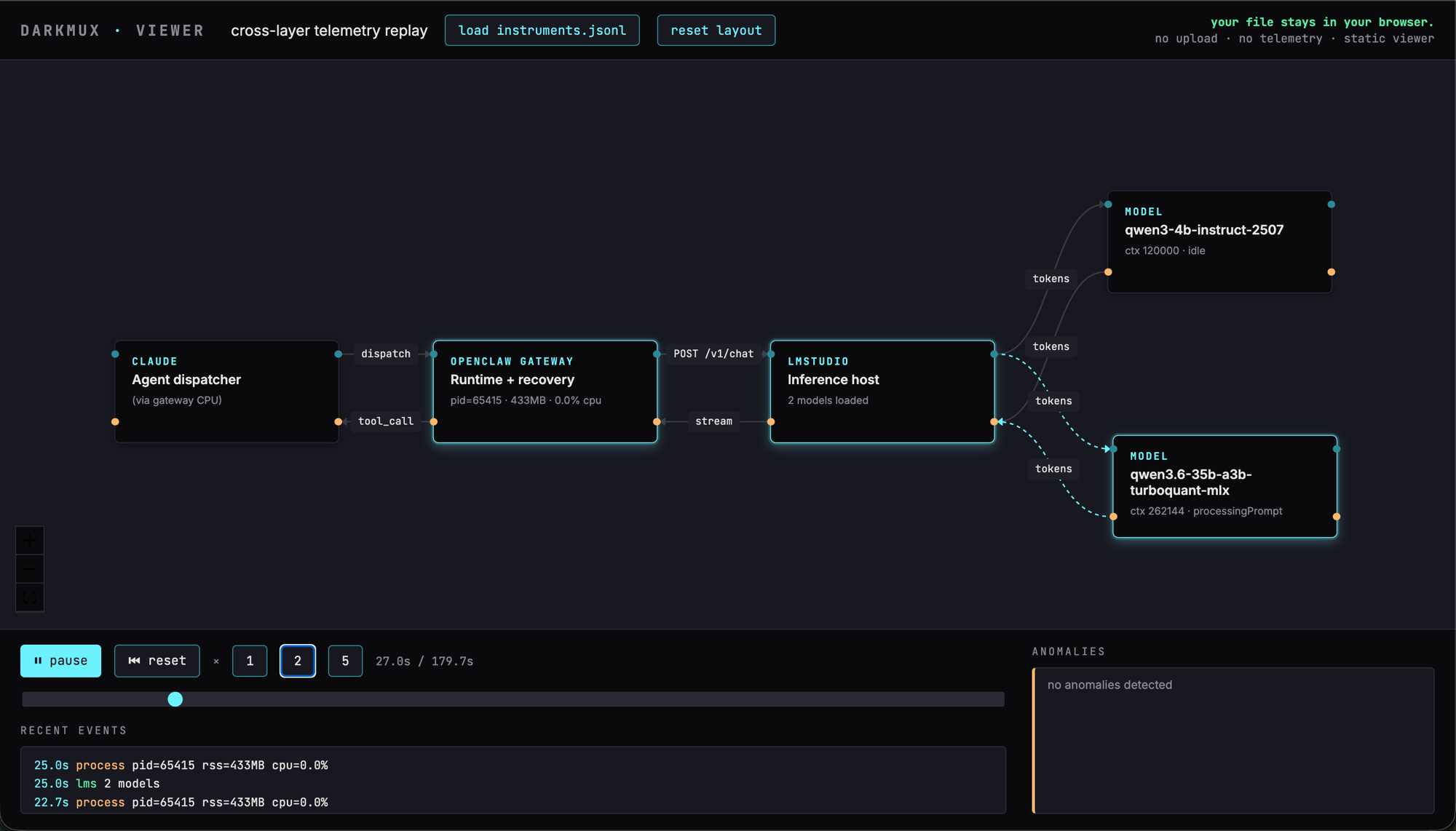
deep profile — qwen3.6-35b primary processing a prompt, qwen3-4b compactor idle. Claude → OpenClaw Gateway → LMStudio backbone runs left-to-right; model nodes branch off the right edge.The viewer is a static page; nothing is uploaded. You drag your instruments.jsonl file onto the window and it runs in your browser. No backend, no telemetry on the telemetry. Anomalies (gateway PID changes during active dispatch, loaded-model-set shifts, missing samplers) are surfaced as call-outs in the bottom panel.
If you want to start running it before Part 3 lands, the project is at darkmux.com. The Quick start gets you from git clone to a working smoke test in about ten minutes, assuming LMStudio is already installed and you’ve downloaded a model. Append --instrument to any lab run and the viewer takes care of the rest.
Go tinker. Stretch your machine, see what surprises you. The runs that don’t match mine are exactly the data Part 3 needs.
Part 3 is in progress. Subscribe to follow the empirical reproduction of these claims on hardware that isn’t mine. The lab notebook is open; the runs are real; the goal is to find the points where this article is wrong, with you.
A note on risk and responsibility
Running local AI — through darkmux or any other tool — means dispatching code on your machine that interacts with your files, runs commands, and consumes system resources outside the protections of a sandbox. You are responsible for your own actions, your own machine, and any work agents do on your behalf.
Configurations validated on my hardware may behave differently on yours. Local-AI workloads can stress thermal limits, exhaust memory, trigger system instability, and produce malformed output that affects downstream systems if you don’t catch the failure yourself. The recommendations here are starting points, not guarantees.
Proceed with caution and at your own risk.
Appendices for operators
The body stuck to the journey. The receipts live here.
Appendix A — Glossary
Context window (or context length, or “loaded context”). How much of the conversation the AI can hold in mind at once, measured in tokens — roughly 3-4 characters of text per token. A 100,000-token context is enough to hold about 75,000 words. Each model has a maximum context it was trained for; the actual operational context is whatever you load it with, which is often less.
Compaction. When the running conversation outgrows the context window, the system summarizes older parts of the conversation to free room. The recent turns are preserved verbatim; the older turns get condensed into a structured summary that the model continues working from. Compaction lets agentic dispatches run for many more turns than would fit in raw context.
Compaction model offload. Running the summarization step on a small dedicated model instead of the main model. The 4-billion-parameter model handling the summary work runs in seconds; if you used the 35B model for both the work AND the summary, every summary would cost a 30+ second beat. Offload splits the labor.
Tool call. A request the AI makes for an action — read this file, run this command, edit these lines. Tool calls are the mechanism by which the assistant interacts with anything outside its own text-generation, and they’re how it reads code, runs tests, writes files, etc.
Agentic dispatch. A multi-step assistant session — the AI makes multiple tool calls, processes their results, and continues working until the task is complete. As distinct from a single-turn Q&A where the assistant produces one response and stops.
Wall clock. Elapsed real time from the start of a dispatch to the end of the assistant’s final response. The metric I care about for operator-facing performance.
Mixture-of-experts (MoE). A model architecture where only a fraction of the parameters activate per token. A 35B-parameter MoE with 3B active params has the capacity of a 35B model and the per-token speed of a 3B model — but still has to load all 35B parameters into memory. Apple Silicon’s unified memory makes this trade-off favorable in a way x86+GPU systems often don’t.
MLX. Apple’s framework for running AI models efficiently on M-series chips. Uses unified memory rather than the GPU-VRAM-shuffle dance traditional in CUDA-land. Most of the performance characteristics in this article are MLX-specific.
Bimodal distribution. A distribution with two distinct peaks rather than one. The fast/slow cluster split discussed in the article is bimodal — there isn’t a “typical” wall-clock for agentic dispatch; there’s fast (one peak) and slow (another peak) with very few measurements in between.
Standing system instructions / preamble. The block of text the runtime prepends to every conversation describing the AI’s identity, how to use its tools, what files it should read for context. The user’s prompt is appended after the preamble.
Appendix B — The configuration receipts
The validated mid-range configuration (called v15.5 in the lab notebook, what I’d recommend as the default for mid-range work on a 35B-A3B MoE on M5 Max + 128 GB):
Loaded context (primary):       101,000 tokens
Loaded context (compactor):     68,000 tokens
contextTokens (runtime budget): 90,000 tokens
compaction.mode:                default
compaction.model:               qwen3-4b-instruct-2507
compaction.maxHistoryShare:     0.35
compaction.recentTurnsPreserve: 5
compaction.customInstructions:  (preserve-verbatim string for
                                 SLAs, version identifiers, file
                                 paths, magic numbers)
The validated long-agentic configuration (called bigctx in the notebook):
Loaded context (primary):       262,144 tokens (model max)
Loaded context (compactor):     120,000 tokens
contextTokens (runtime budget): 250,000 tokens
compaction.*:                   same as v15.5 for the three
                                coupled knobs (maxHistoryShare,
                                recentTurnsPreserve,
                                customInstructions)
The single-variable isolation results (everything else held at v15.5 values):
Variable                        Result
──────────────────────────────  ──────────────────────────────
Compactor context 100K → 68K    Wall clock −50%, quality stable
                                (the free lunch — KV
                                pre-allocation cut, no
                                behavioral effect)

recentTurnsPreserve 5 → 3       Run aborts with context_overflow.
                                Coupled, do not pull.

Drop customInstructions         Run aborts with context_overflow.
                                Coupled, do not pull.

Drop compactor entirely         Wall clock fine on bounded tasks
                                but no protection on long ones.
                                Use only if all your work is
                                bounded.
Hardware on which these are validated: M5 Max, 128 GB unified memory, AC power. Other Apple Silicon RAM tiers (64 GB, 96 GB) need scaled-down variants — see the darkmux project’s m_series_64gb provider for derived (not independently measured) rules.
Compaction trigger thresholds (the math the docs don’t expose)
The runtime documents two compaction modes (default and safeguard) without exposing the actual threshold math. From source-code reading and empirical measurement:
default mode — formula: compaction fires when conversation tokens approach
contextWindow − reserveTokensFloor − softThresholdTokensFor a model loaded with contextWindow=101000, default reserveTokensFloor=20000, default softThresholdTokens=4000 → trigger should be at approximately 77,000 tokens.
default mode — observed: compactions fire earlier in practice — around 39,000 to 43,000 tokens in our measurements, well below the formula prediction. There’s an additional trigger we didn’t fully trace from source — possibly maxHistoryShare-driven, possibly a transcriptBytesProjectedTokens projection heuristic. The takeaway: the documented formula is incomplete; the actual trigger is more eager.
safeguard mode: fires earlier still. Adds tighter guardrails around recent turns (preserving them harder) at the cost of triggering compaction sooner overall.
Why this matters more for local than frontier:
On a 1M-token frontier model, compaction may trigger only once during a long agentic session — after hundreds of turns. The cost of a poor compaction policy is small and effectively invisible.
On a 100K local model, compaction fires repeatedly during a single dispatch. Each fire costs 8–30 seconds (faster when paired with a small dedicated compactor model; slower when the primary handles its own compaction). Mode choice swings wall-clock by 90+ seconds across a long dispatch — a meaningful fraction of total elapsed time on local hardware.
Practical recommendation: set mode: default. Set compaction.model: <small-dedicated-compactor> (e.g. a 4B model). Tune recentTurnsPreserve, maxHistoryShare, and customInstructions as a coupled package — see the validated stack above.
Appendix C — Bugs in detail
1. reserveTokensFloor silent-failure
Setting agents.defaults.compaction.reserveTokensFloor to any non-default value silently breaks the iteration-loop stop signal. Dispatches finish rc=0 but meta.stopReason comes back None, the final assistant message is cut off mid-action, and the agreed-upon structured report never gets generated.
Repro (clean, 3 runs, same prompt + model):
reserveTokensFloor: 20000(default) →stopReason: stop, full structured reportreserveTokensFloor: 95000→stopReason: None, report cut offreserveTokensFloor: 200000→stopReason: None, report cut off
Workaround: don’t set reserveTokensFloor at all. To suppress compaction without triggering this bug, register the truthful loaded contextWindow in the providers list and let the compaction trigger fall under it naturally.
Filing this with a clean repro is a Part 3 prerequisite — flagged in the lab notebook.
2. Harmony-format tool-call parser
OpenClaw’s tool-call parser (in the tool-payload bundle module) doesn’t handle the harmony format used by the gpt-oss-120b model family. Symptom: parse errors on tool emission, dispatches fail with Unexpected end of content or similar. Affects only this model family; other models work fine.
Filed as issue #78326. Resolved upstream by @steipete as commit ba2b033, shipped in v2026.5.9-beta.1. Upgrade if you’re on an older version.
3. systemPromptOverride silently drops workspace files
When systemPromptOverride is set on an agent, the runtime silently excludes AGENTS.md, SOUL.md, IDENTITY.md, USER.md, and TOOLS.md from the prompt because the bootstrap-mode regex only matches BOOTSTRAP.md. The override’s text often references “see your AGENTS.md (loaded below)” creating a dangling reference. Symptom: agent appears to behave inconsistently with project conventions you’ve documented in workspace files.
The fix used here: a small local patch forcing bootstrapMode: "full" in the override path. Must be reapplied after every OpenClaw upgrade.